Before reading this page, please check out the Linear Curve Fitting page . Many of the principles mentioned there will be re-used here, and will not be explained in as much detail.
Calculating The Polynomial Curve
We can write an equation for the error as follows:
e r r = ∑ d i 2 = ( y 1 − f ( x 1 ) ) 2 + ( y 2 − f ( x 2 ) ) 2 + ( y 3 − f ( x 3 ) ) 2 = ∑ i = 1 n ( y i − f ( x i ) ) 2 \begin{align}
err & = \sum d_i^2 \nonumber \\
& = (y_1 - f(x_1))^2 + (y_2 - f(x_2))^2 + (y_3 - f(x_3))^2 \nonumber \\
& = \sum_{i = 1}^{n} (y_i - f(x_i))^2
\end{align} err = ∑ d i 2 = ( y 1 − f ( x 1 ) ) 2 + ( y 2 − f ( x 2 ) ) 2 + ( y 3 − f ( x 3 ) ) 2 = i = 1 ∑ n ( y i − f ( x i ) ) 2 where:n n n x , y x, y x , y f ( x ) f(x) f ( x )
Since we want to fit a polynomial, we can write f ( x ) f(x) f ( x )
f ( x ) = a 0 + a 1 x + a 2 x 2 + . . . + a n x n = a 0 + ∑ j = 1 k a j x j \begin{align}
f(x) &= a_0 + a_1 x + a_2 x^2 + ... + a_n x^n \nonumber \\
&= a_0 + \sum_{j=1}^k a_j x^j
\end{align} f ( x ) = a 0 + a 1 x + a 2 x 2 + ... + a n x n = a 0 + j = 1 ∑ k a j x j where:k k k
Substituting into above:
e r r = ∑ i = 1 n ( y i − ( a 0 + ∑ j = 0 k a j x j ) ) 2 \begin{align}
err = \sum_{i = 1}^{n} (y_i - (a_0 + \sum_{j=0}^k a_j x^j))^2
\end{align} err = i = 1 ∑ n ( y i − ( a 0 + j = 0 ∑ k a j x j ) ) 2 How do we find the minimum of this error function? We use the derivative. If we can differentiate e r r err err
We have k k k a 0 , a 1 , . . . , a k a_0, a_1, ..., a_k a 0 , a 1 , ... , a k
∂ e r r ∂ a 0 = − 2 ∑ i = 1 n ( y i − ( a 0 + ∑ j = 0 k a j x j ) ) = 0 ∂ e r r ∂ a 1 = − 2 ∑ i = 1 n ( y i − ( a 0 + ∑ j = 0 k a j x j ) ) x = 0 ∂ e r r ∂ a 1 = − 2 ∑ i = 1 n ( y i − ( a 0 + ∑ j = 0 k a j x j ) ) x 2 = 0 ⋮ ∂ e r r ∂ a k = − 2 ∑ i = 1 n ( y i − ( a 0 + ∑ j = 0 k a j x j ) ) x k = 0 \begin{align}
\frac{\partial err}{\partial a_0} &= -2 \sum_{i=1}^{n} (y_i - (a_0 + \sum_{j=0}^k a_j x_j)) &= 0 \nonumber \\
\frac{\partial err}{\partial a_1} &= -2 \sum_{i=1}^{n} (y_i - (a_0 + \sum_{j=0}^k a_j x_j))x &= 0 \nonumber \\
\frac{\partial err}{\partial a_1} &= -2 \sum_{i=1}^{n} (y_i - (a_0 + \sum_{j=0}^k a_j x_j))x^2 &= 0 \nonumber \\
\vdots \nonumber \\
\frac{\partial err}{\partial a_k} &= -2 \sum_{i=1}^{n} (y_i - (a_0 + \sum_{j=0}^k a_j x_j))x^k &= 0 \\
\end{align} ∂ a 0 ∂ err ∂ a 1 ∂ err ∂ a 1 ∂ err ⋮ ∂ a k ∂ err = − 2 i = 1 ∑ n ( y i − ( a 0 + j = 0 ∑ k a j x j )) = − 2 i = 1 ∑ n ( y i − ( a 0 + j = 0 ∑ k a j x j )) x = − 2 i = 1 ∑ n ( y i − ( a 0 + j = 0 ∑ k a j x j )) x 2 = − 2 i = 1 ∑ n ( y i − ( a 0 + j = 0 ∑ k a j x j )) x k = 0 = 0 = 0 = 0 These equations can be re-arranged into matrix form:
[ n ∑ x i ∑ x i 2 . . . ∑ x i k ∑ x i ∑ x i 2 ∑ x i 3 . . . ∑ x i k + 1 ∑ x i 2 ∑ x i 3 ∑ x i 4 . . . ∑ x i k + 2 ⋮ ⋮ ⋮ . . . ⋮ ∑ x i k ∑ x i k + 1 ∑ x i k + 2 . . . ∑ x i k + k ] [ a 0 a 1 a 2 ⋮ a k ] = [ ∑ ( y i ) ∑ ( x i y i ) ∑ ( x i 2 y i ) ∑ ( x i k y i ) ] \begin{bmatrix}
n & \sum x_i & \sum x_i^2 & ... & \sum x_i^k \\
\sum x_i & \sum x_i^2 & \sum x_i^3 & ... & \sum x_i^{k+1} \\
\sum x_i^2 & \sum x_i^3 & \sum x_i^4 & ... & \sum x_i^{k+2} \\
\vdots & \vdots & \vdots & ... & \vdots \\
\sum x_i^k & \sum x_i^{k+1} & \sum x_i^{k+2} & ... & \sum x_i^{k+k} \\
\end{bmatrix}
\begin{bmatrix}
a_0 \\ a_1 \\ a_2 \\ \vdots \\ a_k
\end{bmatrix} =
\begin{bmatrix}
\sum (y_i) \\
\sum (x_i y_i) \\
\sum (x_i^2 y_i) \\
\sum (x_i^k y_i)
\end{bmatrix} n ∑ x i ∑ x i 2 ⋮ ∑ x i k ∑ x i ∑ x i 2 ∑ x i 3 ⋮ ∑ x i k + 1 ∑ x i 2 ∑ x i 3 ∑ x i 4 ⋮ ∑ x i k + 2 ... ... ... ... ... ∑ x i k ∑ x i k + 1 ∑ x i k + 2 ⋮ ∑ x i k + k a 0 a 1 a 2 ⋮ a k = ∑ ( y i ) ∑ ( x i y i ) ∑ ( x i 2 y i ) ∑ ( x i k y i ) We solve this by re-arranging (which involves taking the inverse of x \bf{x} x
x = A − 1 B \mathbf{x} = \mathbf{A^{-1}} \mathbf{B} x = A − 1 B
Thus a polynomial curve of best fit is:
y = x [ 0 ] + x [ 1 ] x + x [ 2 ] x 2 + . . . + x [ j ] x j y = x[0] + x[1]x + x[2]x^2 + ... + x[j]x^j y = x [ 0 ] + x [ 1 ] x + x [ 2 ] x 2 + ... + x [ j ] x j
See main.py for Python code which performs these calculations.
Worked Example
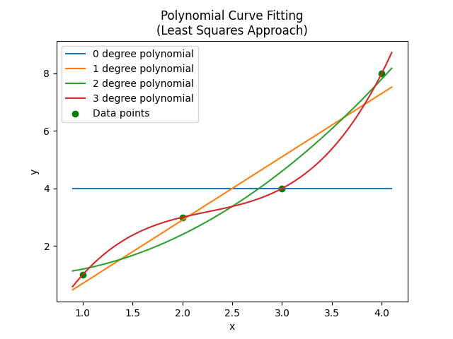
Find a 2 degree polynomial that best describes the following points:
( 1 , 1 ) ( 2 , 3 ) ( 3 , 4 ) ( 4 , 8 ) (1, 1) \\ (2, 3) \\ (3, 4) \\ (4, 8) ( 1 , 1 ) ( 2 , 3 ) ( 3 , 4 ) ( 4 , 8 )
We will then find the values for each one of the nine elements in the A \mathbf{A} A
A 11 = n = 4 A 12 = ∑ x i = 1 + 2 + 3 + 4 = 10 A 13 = ∑ x i 2 = 1 2 + 2 2 + 3 2 + 4 2 = 30 A 21 = A 12 = 10 A 22 = A 13 = 30 A 23 = ∑ x i 3 = 1 3 + 2 3 + 3 3 + 4 3 = 100 A 31 = A 22 = 30 A 32 = A 23 = 100 A 33 = ∑ x i 4 = 1 4 + 2 4 + 3 4 + 4 4 = 354 \begin{align}
A_{11} &= n = 4 \nonumber \\
A_{12} &= \sum x_i = 1 + 2 + 3 + 4 = 10 \nonumber \\
A_{13} &= \sum x_i^2 = 1^2 + 2^2 + 3^2 + 4^2 = 30 \nonumber \\
A_{21} &= A_{12} = 10 \nonumber \\
A_{22} &= A_{13} = 30 \nonumber \\
A_{23} &= \sum x_i^3 = 1^3 + 2^3 + 3^3 + 4^3 = 100 \nonumber \\
A_{31} &= A_{22} = 30 \nonumber \\
A_{32} &= A_{23} = 100 \nonumber \\
A_{33} &= \sum x_i^4 = 1^4 + 2^4 + 3^4 + 4^4 = 354 \\
\end{align} A 11 A 12 A 13 A 21 A 22 A 23 A 31 A 32 A 33 = n = 4 = ∑ x i = 1 + 2 + 3 + 4 = 10 = ∑ x i 2 = 1 2 + 2 2 + 3 2 + 4 2 = 30 = A 12 = 10 = A 13 = 30 = ∑ x i 3 = 1 3 + 2 3 + 3 3 + 4 3 = 100 = A 22 = 30 = A 23 = 100 = ∑ x i 4 = 1 4 + 2 4 + 3 4 + 4 4 = 354 And now find the elements of the B \mathbf{B} B
B 11 = ∑ y i = 1 + 3 + 4 + 8 = 16 B 21 = ∑ x i y i = 1 ∗ 1 + 2 ∗ 3 + 3 ∗ 4 + 4 ∗ 8 = 51 B 31 = ∑ x i 2 y i = 1 2 ∗ 1 + 2 2 ∗ 3 + 3 2 ∗ 4 + 4 2 ∗ 8 = 177 \begin{align}
B_{11} &= \sum y_i = 1 + 3 + 4 + 8 = 16 \nonumber \\
B_{21} &= \sum x_i y_i = 1*1 + 2*3 + 3*4 + 4*8 = 51 \nonumber \\
B_{31} &= \sum x_i^2 y_i = 1^2*1 + 2^2*3 + 3^2*4 + 4^2*8 = 177 \nonumber \\
\end{align} B 11 B 21 B 31 = ∑ y i = 1 + 3 + 4 + 8 = 16 = ∑ x i y i = 1 ∗ 1 + 2 ∗ 3 + 3 ∗ 4 + 4 ∗ 8 = 51 = ∑ x i 2 y i = 1 2 ∗ 1 + 2 2 ∗ 3 + 3 2 ∗ 4 + 4 2 ∗ 8 = 177 Plugging these values into the matrix equation:
[ 4 10 30 10 30 100 30 100 354 ] [ a 0 a 1 a 2 ] = [ 16 51 177 ] \begin{bmatrix}
4 & 10 & 30 \\
10 & 30 & 100 \\
30 & 100 & 354
\end{bmatrix}
\begin{bmatrix}
a_0 \\ a_1 \\ a_2
\end{bmatrix} =
\begin{bmatrix}
16 \\
51 \\
177
\end{bmatrix} 4 10 30 10 30 100 30 100 354 a 0 a 1 a 2 = 16 51 177 We can then solve x = A − 1 B \mathbf{x} = \mathbf{A^{-1}}\mathbf{B} x = A − 1 B
[ a 0 a 1 a 2 ] = [ 1 − 0.3 0.5 ] \begin{bmatrix}a_0 \\ a_1 \\ a_2 \end{bmatrix} =
\begin{bmatrix}1 \\ -0.3 \\ 0.5\end{bmatrix} a 0 a 1 a 2 = 1 − 0.3 0.5 Thus our line of best fit:
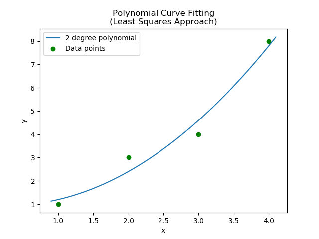
y = 1 − 0.3 x + 0.5 x 2 y = 1 - 0.3x + 0.5x^2 y = 1 − 0.3 x + 0.5 x 2
The data points and polynomial of best fit are shown in the below graph: